Reports Functions¶

This section explains some functions that allows us to create Jupyter Notebook and Excel reports that helps us to analyze quickly the properties of our portfolios.

The following example build an optimum portfolio and create a Jupyter Notebook and Excel report using the functions of this module.

Example¶

import numpy as np
import pandas as pd
import yfinance as yf
import riskfolio as rp

yf.pdr_override()

# Date range
start = '2016-01-01'
end = '2019-12-30'

# Tickers of assets
tickers = ['JCI', 'TGT', 'CMCSA', 'CPB', 'MO', 'APA', 'MRSH', 'JPM',
           'ZION', 'PSA', 'BAX', 'BMY', 'LUV', 'PCAR', 'TXT', 'TMO',
           'DE', 'MSFT', 'HPQ', 'SEE', 'VZ', 'CNP', 'NI', 'T', 'BA']
tickers.sort()

# Downloading the data
data = yf.download(tickers, start = start, end = end)
data = data.loc[:,('Adj Close', slice(None))]
data.columns = tickers
assets = data.pct_change().dropna()

Y = assets

# Creating the Portfolio Object
port = rp.Portfolio(returns=Y)

# To display dataframes values in percentage format
pd.options.display.float_format = '{:.4%}'.format

# Choose the risk measure
rm = 'MV'  # Standard Deviation

# Estimate inputs of the model (historical estimates)
method_mu='hist' # Method to estimate expected returns based on historical data.
method_cov='hist' # Method to estimate covariance matrix based on historical data.

port.assets_stats(method_mu=method_mu, method_cov=method_cov)

# Estimate the portfolio that maximizes the risk adjusted return ratio
w = port.optimization(model='Classic', rm=rm, obj='Sharpe', rf=0.0, l=0, hist=True)

Module Functions¶

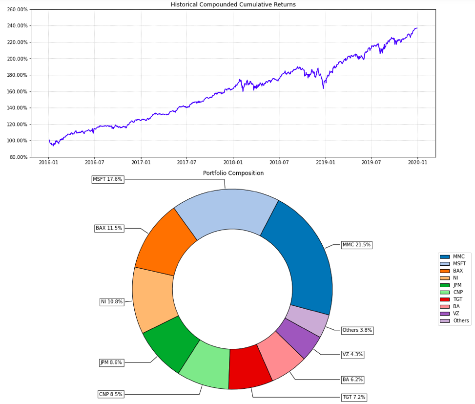
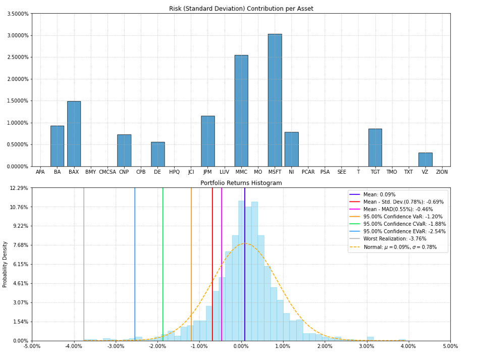
Reports.jupyter_report(returns, w, rm='MV', rf=0, alpha=0.05, a_sim=100, beta=None, b_sim=None, kappa=0.3, solver='CLARABEL', percentage=False, erc_line=True, color='tab:blue', erc_linecolor='r', others=0.05, nrow=25, cmap='tab20', height=6, width=14, t_factor=252, ini_days=1, days_per_year=252, bins=50)[source]¶

Create a matplotlib report with useful information to analyze risk and profitability of investment portfolios.

Parameters:¶

returns : DataFrame of shape (n_samples, n_assets), optional¶

Assets returns DataFrame, where n_samples is the number of observations and n_assets is the number of assets.

w : DataFrame or Series of shape (n_assets, 1)¶

Portfolio weights, where n_assets is the number of assets.

rm : str, optional¶

Risk measure used to estimate risk contribution. The default is ‘MV’. Possible values are:

’MV’: Standard Deviation.
’KT’: Square Root Kurtosis.
’MAD’: Mean Absolute Deviation.
’GMD’: Gini Mean Difference.
’MSV’: Semi Standard Deviation.
’SKT’: Square Root Semi Kurtosis.
’FLPM’: First Lower Partial Moment (Omega Ratio).
’SLPM’: Second Lower Partial Moment (Sortino Ratio).
’CVaR’: Conditional Value at Risk.
’TG’: Tail Gini.
’EVaR’: Entropic Value at Risk.
’RLVaR’: Relativistc Value at Risk.
’WR’: Worst Realization (Minimax).
’CVRG’: CVaR range of returns.
’TGRG’: Tail Gini range of returns.
’RG’: Range of returns.
’MDD’: Maximum Drawdown of uncompounded cumulative returns (Calmar Ratio).
’ADD’: Average Drawdown of uncompounded cumulative returns.
’DaR’: Drawdown at Risk of uncompounded cumulative returns.
’CDaR’: Conditional Drawdown at Risk of uncompounded cumulative returns.
’EDaR’: Entropic Drawdown at Risk of uncompounded cumulative returns.
’RLDaR’: Relativistic Drawdown at Risk of uncompounded cumulative returns.
’UCI’: Ulcer Index of uncompounded cumulative returns.

rf : float, optional¶

Risk free rate or minimum acceptable return. The default is 0.

alpha : float, optional¶

Significance level of VaR, CVaR, Tail Gini, EVaR, RLVaR, CDaR, EDaR and RLDaR. The default is 0.05. The default is 0.05.

a_sim : float, optional¶

Number of CVaRs used to approximate Tail Gini of losses. The default is 100.

beta : float, optional¶

Significance level of CVaR and Tail Gini of gains. If None it duplicates alpha value. The default is None.

b_sim : float, optional¶

Number of CVaRs used to approximate Tail Gini of gains. If None it duplicates a_sim value. The default is None.

kappa : float, optional¶

Deformation parameter of RLVaR and RLDaR, must be between 0 and 1. The default is 0.30.

solver : str, optional¶

Solver available for CVXPY that supports power cone programming and exponential cone programming. Used to calculate EVaR, EDaR, RLVaR and RLDaR. The default value is ‘CLARABEL’.

percentage : bool, optional¶

If risk contribution per asset is expressed as percentage or as a value. The default is False.

erc_line : bool, optional¶

If equal risk contribution line is plotted. The default is False.

color : str, optional¶

Color used to plot each asset risk contribution. The default is ‘tab:blue’.

erc_linecolor : str, optional¶

Color used to plot equal risk contribution line. The default is ‘r’.

others : float, optional¶

Percentage of others section. The default is 0.05.

nrow : int, optional¶

Number of rows of the legend. The default is 25.

cmap : cmap, optional¶

Color scale used to plot each asset weight. The default is ‘tab20’.

height : float, optional¶

Average height of charts in the image in inches. The default is 6.

width : float, optional¶

Width of the image in inches. The default is 14.

t_factor : float, optional¶

Factor used to annualize expected return and expected risks for risk measures based on returns (not drawdowns). The default is 252.

\[\begin{split}\begin{align} \text{Annualized Return} & = \text{Return} \, \times \, \text{t_factor} \\ \text{Annualized Risk} & = \text{Risk} \, \times \, \sqrt{\text{t_factor}} \end{align}\end{split}\]

ini_days : float, optional¶

If provided, it is the number of days of compounding for first return. It is used to calculate Compound Annual Growth Rate (CAGR). This value depend on assumptions used in t_factor, for example if data is monthly you can use 21 (252 days per year) or 30 (360 days per year). The default is 1 for daily returns.

days_per_year : float, optional¶

Days per year assumption. It is used to calculate Compound Annual Growth Rate (CAGR). Default value is 252 trading days per year.

bins : float, optional¶

Number of bins of the histogram. The default is 50.

Raises:¶

ValueError – When the value cannot be calculated.

Returns:¶

ax – Returns the Axes object with the plot for further tweaking.

Return type:¶

matplotlib axis of size (6,1)

Example

ax = rp.jupyter_report(returns,
                       w,
                       rm='MV',
                       rf=0,
                       alpha=0.05,
                       height=6,
                       width=14,
                       others=0.05,
                       nrow=25)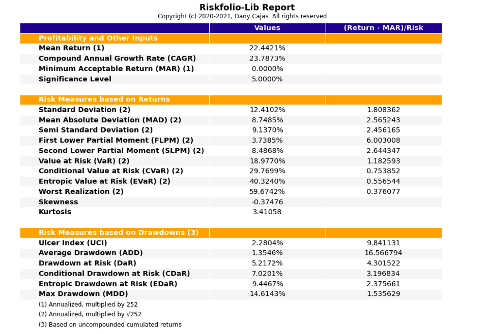

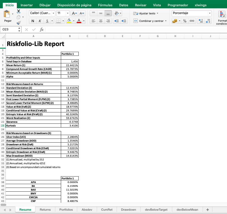
Reports.excel_report(returns, w, rf=0, alpha=0.05, solver='CLARABEL', t_factor=252, ini_days=1, days_per_year=252, name='report')[source]¶

Create an Excel report (with formulas) with useful information to analyze risk and profitability of investment portfolios.