Constraints Functions¶

This module has functions that help users to create linear and integer constraints related to the assets, assets classes or risk factors.

This module have functions that help users to create assets and factors views for the Black Litterman model [E1], Augmented Black Litterman [E2], Black Litterman Bayes [E3], and the Entropy Pooling model [E4].

This module also have functions to create constraints based on graph information [E5] and [E6] like the information obtained from networks and dendrograms.

Module Functions¶

ConstraintsFunctions.assets_constraints(constraints, asset_classes)[source]¶

Create the linear constraints matrices A and B of the constraint \(Aw \leq B\).

Parameters:¶

constraints : DataFrame of shape (n_constraints, n_fields)¶

Constraints DataFrame, where n_constraints is the number of constraints and n_fields is the number of fields of constraints DataFrame, the fields are:

• Disabled: (bool) indicates if the constraint is enable.

• Type: (str) can be ‘Assets’, ‘Classes’, ‘All Assets’, ‘Each asset in a class’ and ‘All Classes’.

• Set: (str) if Type is ‘Classes’, ‘Each asset in a class’ or ‘All Classes’ specified the name of the asset’s classes set.

• Position: (str) the name of the asset or asset class of the constraint.

• Sign: (str) can be ‘>=’ or ‘<=’.

• Weight: (scalar) is the maximum or minimum weight of the absolute constraint.

• Type Relative: (str) can be ‘Assets’ or ‘Classes’.

• Relative Set: (str) if Type Relative is ‘Classes’ specified the name of the set of asset classes.

• Relative: (str) the name of the asset or asset class of the relative constraint.

• Factor: (scalar) is the factor of the relative constraint.

asset_classes : DataFrame of shape (n_assets, n_cols)¶

Asset’s classes matrix, where n_assets is the number of assets and n_cols is the number of columns of the matrix where the first column is the asset list and the next columns are the different asset’s classes sets.

Returns:¶

• A (nd-array) – The matrix A of \(Aw \leq B\).

• B (nd-array) – The matrix B of \(Aw \leq B\).

Raises:¶

ValueError when the value cannot be calculated. –

Examples

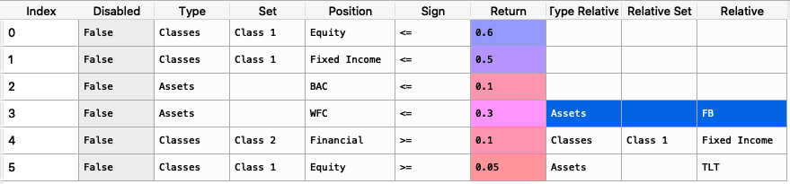
import riskfolio as rp

asset_classes = {'Assets': ['META', 'GOOGL', 'NFLX', 'BAC', 'WFC', 'TLT', 'SHV'],
                 'Class 1': ['Equity', 'Equity', 'Equity', 'Equity', 'Equity',
                             'Fixed Income', 'Fixed Income'],
                 'Class 2': ['Technology', 'Technology', 'Technology',
                             'Financial', 'Financial', 'Treasury', 'Treasury'],}

asset_classes = pd.DataFrame(asset_classes)
asset_classes = asset_classes.sort_values(by=['Assets'])

constraints = {'Disabled': [False, False, False, False, False, False, False],
               'Type': ['Classes', 'Classes', 'Assets', 'Assets', 'Classes',
                        'All Assets', 'Each asset in a class'],
               'Set': ['Class 1', 'Class 1', '', '', 'Class 2', '', 'Class 1'],
               'Position': ['Equity', 'Fixed Income', 'BAC', 'WFC', 'Financial',
                            '', 'Equity'],
               'Sign': ['<=', '<=', '<=', '<=', '>=', '>=', '>='],
               'Weight': [0.6, 0.5, 0.1, '', '', 0.02, ''],
               'Type Relative': ['', '', '', 'Assets', 'Classes', '', 'Assets'],
               'Relative Set': ['', '', '', '', 'Class 1', '', ''],
               'Relative': ['', '', '', 'META', 'Fixed Income', '', 'TLT'],
               'Factor': ['', '', '', 1.2, 0.5, '', 0.4]}

constraints = pd.DataFrame(constraints)

The constraints look like the following image:

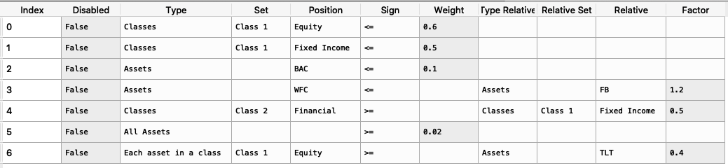
It is easier to construct the constraints in excel and then upload to a dataframe.

To create the matrices A and B we use the following command:

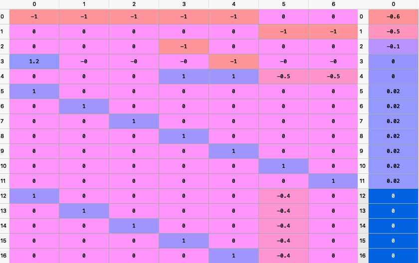
A, B = rp.assets_constraints(constraints, asset_classes)

The matrices A and B looks like this (all constraints were converted to a linear constraint):

ConstraintsFunctions.factors_constraints(constraints, loadings)[source]¶

Create the factors constraints matrices C and D of the constraint \(Cw \leq D\).

Parameters:¶

constraints : DataFrame of shape (n_constraints, n_fields)¶

Constraints DataFrame, where n_constraints is the number of constraints and n_fields is the number of fields of constraints DataFrame, the fields are:

• Disabled: (bool) indicates if the constraint is enable.

• Factor: (str) the name of the factor of the constraint.

• Sign: (str) can be ‘>=’ or ‘<=’.

• Value: (scalar) is the maximum or minimum value of the factor.

loadings : DataFrame of shape (n_assets, n_features)¶

The loadings matrix.

Returns:¶

• C (nd-array) – The matrix C of \(Cw \leq D\).

• D (nd-array) – The matrix D of \(Cw \leq D\).

Raises:¶

ValueError when the value cannot be calculated. –

Examples

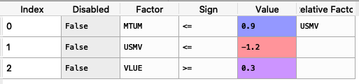
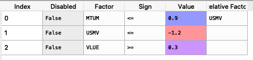
loadings = {'const': [0.0004, 0.0002, 0.0000, 0.0006, 0.0001, 0.0003, -0.0003],
            'MTUM': [0.1916, 1.0061, 0.8695, 1.9996, 0.0000, 0.0000, 0.0000],
            'QUAL': [0.0000, 2.0129, 1.4301, 0.0000, 0.0000, 0.0000, 0.0000],
            'SIZE': [0.0000, 0.0000, 0.0000, 0.4717, 0.0000, -0.1857, 0.0000],
            'USMV': [-0.7838, -1.6439, -1.0176, -1.4407, 0.0055, 0.5781, 0.0000],
            'VLUE': [1.4772, -0.7590, -0.4090, 0.0000, -0.0054, -0.4844, 0.9435]}

loadings = pd.DataFrame(loadings)

constraints = {'Disabled': [False, False, False],
               'Factor': ['MTUM', 'USMV', 'VLUE'],
               'Sign': ['<=', '<=', '>='],
               'Value': [0.9, -1.2, 0.3],
               'Relative Factor': ['USMV', '', '']}

constraints = pd.DataFrame(constraints)

The constraints look like the following image:

It is easier to construct the constraints in excel and then upload to a dataframe.

To create the matrices C and D we use the following command:

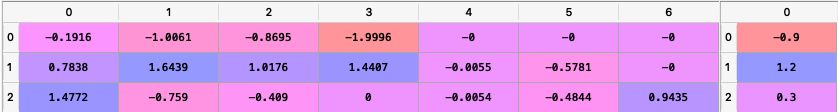
C, D = rp.factors_constraints(constraints, loadings)

The matrices C and D looks like this (all constraints were converted to a linear constraint):

ConstraintsFunctions.integer_constraints(constraints, asset_classes)[source]¶

Create the integer constraints matrices A, B, C, D, E, F associated to the constraints \(Ak \leq B\), \(Ck \leq D \odot k_{s}\) and \(E k_{s}\leq F\).

Parameters:¶

constraints : DataFrame of shape (n_constraints, n_fields)¶

Constraints DataFrame, where n_constraints is the number of constraints and n_fields is the number of fields of constraints DataFrame, the fields are:

• Disabled: (bool) indicates if the constraint is enable.

• Type: (str) can be ‘Assets’ and ‘Classes’.

• Set: (str) if Type is ‘Classes’ specified the name of the asset’s classes set.

• Position: (str) the name of the asset or asset class of the constraint, or ‘All’ for all categories.

• Kind: (str) can be ‘CardUp’ (Upper Cardinality), ‘CardLow’ (Lower Cardinality), ‘MuEx’ (Mutually Exclusive) and ‘Join’ (Join Investments).

• Value: (int or None) is the maximum or minimum value of cardinality constraints.

• Type Relative: (str) can be: ‘Assets’ or ‘Classes’.

• Relative Set: (str) if Type Relative is ‘Classes’ specified the name of the set of asset classes.

• Relative: (str) the name of the asset or asset class of the relative constraint.

asset_classes : DataFrame of shape (n_assets, n_cols)¶

Asset’s classes matrix, where n_assets is the number of assets and n_cols is the number of columns of the matrix where the first column is the asset list and the next columns are the different asset’s classes sets.

Returns:¶

• A (dict) – The dictionary that containts the matrices A of \(Ak \leq B\).

• B (dict) – The dictionary that containts the matrices B of \(Ak \leq B\).

• C (dict) – The dictionary that containts the matrices C of \(Ck \leq D \odot k_{s}\).

• D (dict) – The dictionary that containts the matrices D of \(Ck \leq D \odot k_{s}\).

• E (dict) – The dictionary that containts the matrices E of \(E k_{s}\leq F\).

• F (dict) – The dictionary that containts the matrices F of \(E k_{s}\leq F\).

Raises:¶

ValueError when the value cannot be calculated. –

Examples

import riskfolio as rp

asset_classes = {'Assets': ['META', 'GOOGL', 'NFLX', 'BAC', 'WFC', 'TLT', 'SHV'],
                 'Class 1': ['Equity', 'Equity', 'Equity', 'Equity', 'Equity',
                             'Fixed Income', 'Fixed Income'],
                 'Class 2': ['Technology', 'Technology', 'Technology',
                             'Financial', 'Financial', 'Treasury', 'Treasury'],}

asset_classes = pd.DataFrame(asset_classes)
asset_classes = asset_classes.sort_values(by=['Assets'])

constraints = {'Disabled': [False, False, False, False, False, False, False, False, False, False, False, False],
               'Type': ['Assets', 'Assets', 'Assets', 'Assets', 'Classes', 'Classes', 'Classes', 'Classes', 'Classes', 'Classes', 'Classes', 'Classes'],
               'Set': ['', '', '', '', 'Class 2', 'Class 2', 'Class 2', 'Class 2', 'Class 2', 'Class 2', 'Class 2', 'Class 2'],
               'Position': ['', '', 'META', 'TLT', '', '', 'Financial', 'Technology', 'Financial', 'Financial', 'Treasury', 'Treasury'],
               'Kind': ['CardUp', 'CardLow', 'MuEx', 'Join', 'CardUp', 'CardLow', 'CardUp', 'CardLow', 'MuEx', 'MuEx', 'Join', 'Join'],
               'Value': [4.0, 3.0, '', '', 1.0, 2.0, 1.0, 1.0, '', '', '', ''],
               'Type Relative': ['', '', 'Assets', 'Assets', '', '', '', '', 'Assets', 'Classes', 'Assets', 'Classes'],
               'Relative Set': ['', '', '', '', '', '', '', '', '', 'Class 2', '', 'Class 2'],
               'Relative': ['', '', 'BAC', 'GOOGL', '', '', '', '', 'TLT', 'Financial', 'BAC', 'Technology']}
constraints = pd.DataFrame(constraints)

The constraints look like the following image:

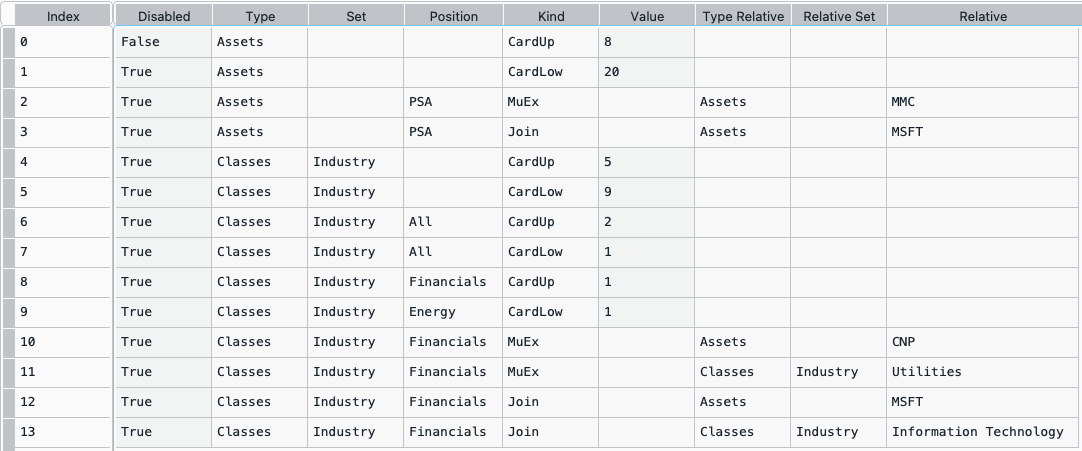
It is easier to construct the constraints in excel and then upload to a dataframe.

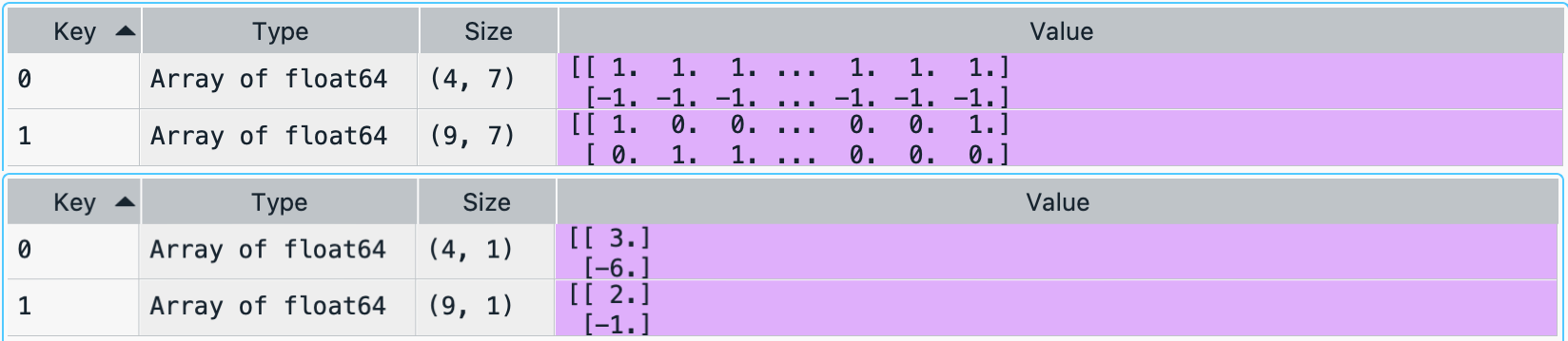
To create the dictionaries A, B, C, D, E, and F we use the following command:

A, B, C, D, E, F = rp.integer_constraints(constraints, asset_classes)

The dictionaries A and B look like the following image:

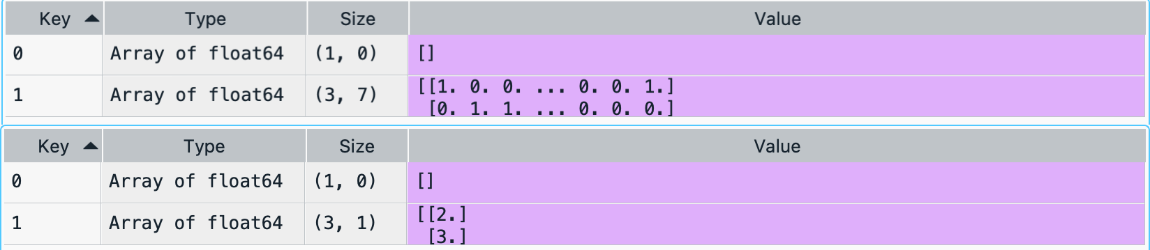
The dictionaries C and D look like the following image:

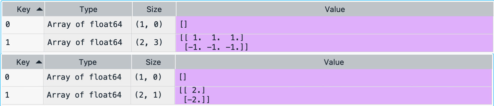
The dictionaries E and F look like the following image:

ConstraintsFunctions.assets_views(views, asset_classes)[source]¶

Create the assets views matrices P and Q of the views \(Pw = Q\).

Parameters:¶

views : DataFrame of shape (n_views, n_fields)¶

views DataFrame, where n_views is the number of views and n_fields is the number of fields of views DataFrame, the fields are:

• Disabled: (bool) indicates if the constraint is enable.

• Type: (str) can be: ‘Assets’ or ‘Classes’.

• Set: (str) if Type is ‘Classes’ specified the name of the set of asset classes.

• Position: (str) the name of the asset or asset class of the view.

• Sign: (str) can be ‘>=’ or ‘<=’.

• Return: (scalar) is the return of the view.

• Type Relative: (str) can be: ‘Assets’ or ‘Classes’.

• Relative Set: (str) if Type Relative is ‘Classes’ specified the name of the set of asset classes.

• Relative: (str) the name of the asset or asset class of the relative view.

asset_classes : DataFrame of shape (n_assets, n_cols)¶

Asset’s classes matrix, where n_assets is the number of assets and n_cols is the number of columns of the matrix where the first column is the asset list and the next columns are the different asset’s classes sets.

Returns:¶

• P (nd-array) – The matrix P that shows the relation among assets in each view.

• Q (nd-array) – The matrix Q that shows the expected return of each view.

Raises:¶

ValueError when the value cannot be calculated. –

Examples

asset_classes = {'Assets': ['META', 'GOOGL', 'NFLX', 'BAC', 'WFC', 'TLT', 'SHV'],
                 'Class 1': ['Equity', 'Equity', 'Equity', 'Equity', 'Equity',
                              'Fixed Income', 'Fixed Income'],
                 'Class 2': ['Technology', 'Technology', 'Technology',
                              'Financial', 'Financial', 'Treasury', 'Treasury'],}

asset_classes = pd.DataFrame(asset_classes)
asset_classes = asset_classes.sort_values(by=['Assets'])

views = {'Disabled': [False, False, False, False],
         'Type': ['Assets', 'Classes', 'Classes', 'Assets'],
         'Set': ['', 'Class 2','Class 1', ''],
         'Position': ['WFC', 'Financial', 'Equity', 'META'],
         'Sign': ['<=', '>=', '>=', '>='],
         'Return': [ 0.3, 0.1, 0.05, 0.03 ],
         'Type Relative': [ 'Assets', 'Classes', 'Assets', ''],
         'Relative Set': [ '', 'Class 1', '', ''],
         'Relative': ['META', 'Fixed Income', 'TLT', '']}

views = pd.DataFrame(views)

The constraints look like the following image:

It is easier to construct the constraints in excel and then upload to a dataframe.

To create the matrices P and Q we use the following command:

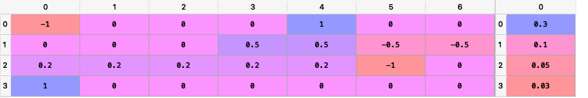
P, Q = rp.assets_views(views, asset_classes)

The matrices P and Q look like the following image:

ConstraintsFunctions.factors_views(views, loadings, const=True)[source]¶

Create the factors constraints matrices C and D of the constraint \(Cw \geq D\).

Parameters:¶

views : DataFrame of shape (n_views, n_fields)¶

views DataFrame, where n_views is the number of views and n_fields is the number of fields of views DataFrame, the fields are:

• Disabled: (bool) indicates if the constraint is enable.

• Factor: (str) the name of the factor of the constraint.

• Sign: (str) can be ‘>=’ or ‘<=’.

• Value: (scalar) is the maximum or minimum value of the factor.

loadings : DataFrame of shape (n_assets, n_features)¶

The loadings matrix.

Returns:¶

• P (nd-array) – The matrix P that shows the relation among factors in each factor view.

• Q (nd-array) – The matrix Q that shows the expected return of each factor view.

Raises:¶

ValueError when the value cannot be calculated. –

Examples

loadings = {'const': [0.0004, 0.0002, 0.0000, 0.0006, 0.0001, 0.0003, -0.0003],
            'MTUM': [0.1916, 1.0061, 0.8695, 1.9996, 0.0000, 0.0000, 0.0000],
            'QUAL': [0.0000, 2.0129, 1.4301, 0.0000, 0.0000, 0.0000, 0.0000],
            'SIZE': [0.0000, 0.0000, 0.0000, 0.4717, 0.0000, -0.1857, 0.0000],
            'USMV': [-0.7838, -1.6439, -1.0176, -1.4407, 0.0055, 0.5781, 0.0000],
            'VLUE': [1.4772, -0.7590, -0.4090, 0.0000, -0.0054, -0.4844, 0.9435]}

loadings = pd.DataFrame(loadings)

factorsviews = {'Disabled': [False, False, False],
                'Factor': ['MTUM', 'USMV', 'VLUE'],
                'Sign': ['<=', '<=', '>='],
                'Value': [0.9, -1.2, 0.3],
                'Relative Factor': ['USMV', '', '']}

factorsviews = pd.DataFrame(factorsviews)

The constraints look like the following image:

It is easier to construct the constraints in excel and then upload to a dataframe.

To create the matrices P and Q we use the following command:

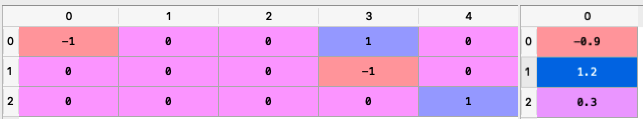
P, Q = rp.factors_views(factorsviews,
                        loadings,
                        const=True)

The matrices P and Q look like the following image:

ConstraintsFunctions.entropy_pooling_views(views: DataFrame, asset_classes: DataFrame, returns: DataFrame)[source]¶

Create the linear constraints matrices P_eq, Q_eq, P_in and Q_in of the constraint \(P_{eq} Z = Q_{eq}\) and \(P_{in} Z \geq Q_{in}\).

Parameters:¶

views : pd.DataFrame of shape (n_views, n_fields)¶

views DataFrame, where n_views is the number of views and n_fields is the number of fields of views DataFrame, the fields are:

• Disabled: (bool) indicates if the constraint is enable.

• Kind: (str) can be: ‘Mean’, ‘Var’, ‘Covar’, ‘Corr’, ‘Skew’ and ‘Kurt’.

• Type: (str) can be: ‘Assets’ or ‘Classes’. Type ‘Classes’ is only available for kind ‘Mean’.

• Set: (str) if Type is ‘Classes’ specified the name of the set of asset classes.

• Position: (str) the name of the asset or asset class of the view.

• Sign: (str) can be ‘>=’, ‘==’ or ‘<=’. Sign ‘<=’ is only available for kind ‘Mean’.

• Return: (scalar) is the return of the view.

• Type Relative: (str) can be: ‘Assets’ or ‘Classes’. Type ‘Classes’ is only available for kind ‘Mean’.

• Relative Set: (str) if Type Relative is ‘Classes’ specified the name of the set of asset classes.

• Relative: (str) the name of the asset or asset class of the relative view.

asset_classes : pd.DataFrame of shape (n_assets, n_cols)¶

Asset’s classes matrix, where n_assets is the number of assets and n_cols is the number of columns of the matrix where the first column is the asset list and the next columns are the different asset’s classes sets.

returns : pd.DataFrame of shape (n_samples, n_assets)¶

Assets returns DataFrame, where n_samples is the number of observations and n_assets is the number of assets.

Returns:¶

• P_eq (np.ndarray) – Matrix P of equality constraint \(P_{eq} Z = Q_{eq}\).

• Q_eq (np.ndarray) – Matrix Q of equality constraint \(P_{eq} Z = Q_{eq}\).

• P_in (np.ndarray) – Matrix P of inequality constraint \(P_{eq} Z \geq Q_{eq}\).

• Q_in (np.ndarray) – Matrix Q of inequality constraint \(P_{eq} Z \geq Q_{eq}\).

Raises:¶

ValueError when the value cannot be calculated. –

Examples

asset_classes = {'Assets': ['META', 'GOOGL', 'NFLX', 'BAC', 'WFC', 'TLT', 'SHV'],
                 'Class 1': ['Equity', 'Equity', 'Equity', 'Equity', 'Equity',
                              'Fixed Income', 'Fixed Income'],
                 'Class 2': ['Technology', 'Technology', 'Technology',
                              'Financial', 'Financial', 'Treasury', 'Treasury'],}

asset_classes = pd.DataFrame(asset_classes)
asset_classes = asset_classes.sort_values(by=['Assets'])

views = {'Disabled': [False, True, True, True, True, False, False, False],
         'Kind':['Mean', 'Mean', 'Mean', 'Std', 'Covar', 'Corr', 'Skew', 'Kurt'],
         'Type': ['Assets', 'Assets', 'Assets', 'Assets', 'Assets', 'Assets',
                  'Assets', 'Assets'],
         'Set': ['', '', '', '', '', '', '', ''],
         'Position': ['BAC', 'BAC', 'BAC', 'BAC', 'BAC', 'BAC', 'BAC', 'BAC'],
         'Sign': ['==', '>=', '>=', '==', '==', '==', '==', '=='],
         'Weight': [0.0006, 0.0008, 0.0008, 0.04, 0.0009, 0.7, 0.5, 4],
         'Type Relative': ['', 'Assets', 'Classes', '', 'Assets', 'Assets', '', ''],
         'Relative Set': ['', '', 'Class 2', '', '', '', '', ''],
         'Relative': ['', 'TLT', 'Treasury', '', 'GOOGL', 'GOOGL', '', ''],
         'Factor': ['', '', '', '', '', '', '', '']
         }

views = pd.DataFrame(views)

The constraints look like the following image:

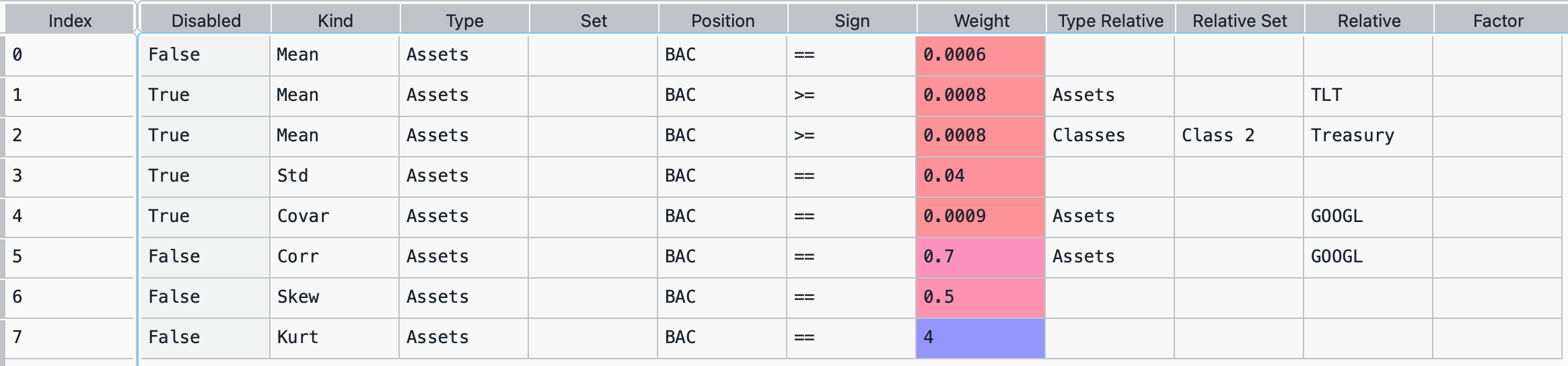
It is easier to construct the constraints in excel and then upload to a dataframe.

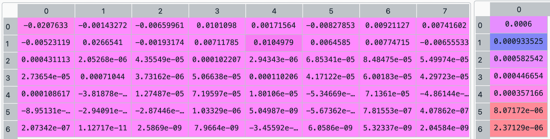
To create the matrices P and Q we use the following command:

P_eq, Q_eq, P_in, Q_in = rp.assets_views(views, asset_classes)

The matrices P_eq and Q_eq, and P_in and Q_in look like the following image:

ConstraintsFunctions.assets_clusters(returns, custom_cov=None, codependence='pearson', linkage='ward', opt_k_method='twodiff', k=None, max_k=10, bins_info='KN', alpha_tail=0.05, gs_threshold=0.5, leaf_order=True)[source]¶

Create asset classes based on hierarchical clustering.

Parameters:¶

returns : DataFrame of shape (n_samples, n_assets)¶

Assets returns DataFrame, where n_samples is the number of observations and n_assets is the number of assets.

custom_cov : DataFrame or None, optional¶

Custom covariance matrix, used when codependence parameter has value ‘custom_cov’. The default is None.

codependence : str, can be {'pearson', 'spearman', 'abs_pearson', 'abs_spearman', 'distance', 'mutual_info', 'tail' or 'custom_cov'}¶

The codependence or similarity matrix used to build the distance metric and clusters. The default is ‘pearson’. Possible values are:

• ’pearson’: pearson correlation matrix. Distance formula: \(D_{i,j} = \sqrt{0.5(1-\rho^{pearson}_{i,j})}\).

• ’spearman’: spearman correlation matrix. Distance formula: \(D_{i,j} = \sqrt{0.5(1-\rho^{spearman}_{i,j})}\).

• ’kendall’: kendall correlation matrix. Distance formula: \(D_{i,j} = \sqrt{0.5(1-\rho^{kendall}_{i,j})}\).

• ’gerber1’: Gerber statistic 1 correlation matrix. Distance formula: \(D_{i,j} = \sqrt{0.5(1-\rho^{gerber1}_{i,j})}\).

• ’gerber2’: Gerber statistic 2 correlation matrix. Distance formula: \(D_{i,j} = \sqrt{0.5(1-\rho^{gerber2}_{i,j})}\).

• ’abs_pearson’: absolute value pearson correlation matrix. Distance formula: \(D_{i,j} = \sqrt{(1-|\rho_{i,j}|)}\).

• ’abs_spearman’: absolute value spearman correlation matrix. Distance formula: \(D_{i,j} = \sqrt{(1-|\rho_{i,j}|)}\).

• ’abs_kendall’: absolute value kendall correlation matrix. Distance formula: \(D_{i,j} = \sqrt{(1-|\rho^{kendall}_{i,j}|)}\).

• ’distance’: distance correlation matrix. Distance formula \(D_{i,j} = \sqrt{(1-\rho^{distance}_{i,j})}\).

• ’mutual_info’: mutual information matrix. Distance used is variation information matrix.

• ’tail’: lower tail dependence index matrix. Dissimilarity formula \(D_{i,j} = -\log{\lambda_{i,j}}\).

• ’custom_cov’: use custom correlation matrix based on the custom_cov parameter. Distance formula: \(D_{i,j} = \sqrt{0.5(1-\rho^{pearson}_{i,j})}\).

linkage : string, optional¶

Linkage method of hierarchical clustering, see linkage for more details. The default is ‘ward’. Possible values are:

• ’single’.

• ’complete’.

• ’average’.

• ’weighted’.

• ’centroid’.

• ’median’.

• ’ward’.

• ’DBHT’. Direct Bubble Hierarchical Tree.

opt_k_method : str¶

Method used to calculate the optimum number of clusters. The default is ‘twodiff’. Possible values are:

• ’twodiff’: two difference gap statistic.

• ’stdsil’: standarized silhouette score.

k : int, optional¶

Number of clusters. This value is took instead of the optimal number of clusters calculated with the two difference gap statistic. The default is None.

max_k : int, optional¶

Max number of clusters used by the two difference gap statistic to find the optimal number of clusters. The default is 10.

bins_info : int or str¶

Number of bins used to calculate variation of information. The default value is ‘KN’. Possible values are:

• ’KN’: Knuth’s choice method. See more in knuth_bin_width.

• ’FD’: Freedman–Diaconis’ choice method. See more in freedman_bin_width.

• ’SC’: Scotts’ choice method. See more in scott_bin_width.

• ’HGR’: Hacine-Gharbi and Ravier’ choice method.

• int: integer value choice by user.

alpha_tail : float, optional¶

Significance level for lower tail dependence index. The default is 0.05.

gs_threshold : float, optional¶

Gerber statistic threshold. The default is 0.5.

leaf_order : bool, optional¶

Indicates if the cluster are ordered so that the distance between successive leaves is minimal. The default is True.

Returns:¶

clusters – A dataframe with asset classes based on hierarchical clustering.

Return type:¶

DataFrame

Raises:¶

ValueError when the value cannot be calculated. –

Examples

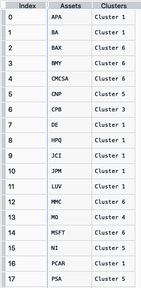
clusters = rp.assets_clusters(returns,
                              codependence='pearson',
                              linkage='ward',
                              k=None,
                              max_k=10,
                              alpha_tail=0.05,
                              leaf_order=True)

The clusters dataframe looks like the following image:

ConstraintsFunctions.hrp_constraints(constraints, asset_classes)[source]¶

Create the upper and lower bounds constraints for hierarchical risk parity model.

Parameters:¶

constraints : DataFrame of shape (n_constraints, n_fields)¶

Constraints DataFrame, where n_constraints is the number of constraints and n_fields is the number of fields of constraints DataFrame, the fields are:

• Disabled: (bool) indicates if the constraint is enable.

• Type: (str) can be: ‘Assets’, All Assets’ and ‘Each asset in a class’.

• Position: (str) the name of the asset or asset class of the constraint.

• Sign: (str) can be ‘>=’ or ‘<=’.

• Weight: (scalar) is the maximum or minimum weight of the absolute constraint.

asset_classes : DataFrame of shape (n_assets, n_cols)¶

Asset’s classes DataFrame, where n_assets is the number of assets and n_cols is the number of columns of the DataFrame where the first column is the asset list and the next columns are the different asset’s classes sets.

Returns:¶

• w_max (pd.Series) – The upper bound of hierarchical risk parity weights constraints.

• w_min (pd.Series) – The lower bound of hierarchical risk parity weights constraints.

Raises:¶

ValueError when the value cannot be calculated. –

Examples

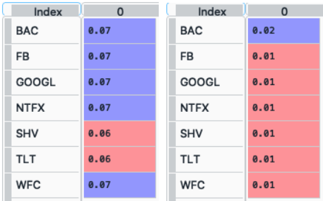
asset_classes = {'Assets': ['META', 'GOOGL', 'NFLX', 'BAC', 'WFC', 'TLT', 'SHV'],
                 'Class 1': ['Equity', 'Equity', 'Equity', 'Equity', 'Equity',
                             'Fixed Income', 'Fixed Income'],
                 'Class 2': ['Technology', 'Technology', 'Technology',
                             'Financial', 'Financial', 'Treasury', 'Treasury'],}

asset_classes = pd.DataFrame(asset_classes)
asset_classes = asset_classes.sort_values(by=['Assets'])

constraints = {'Disabled': [False, False, False, False, False, False],
               'Type': ['Assets', 'Assets', 'All Assets', 'All Assets',
                        'Each asset in a class', 'Each asset in a class'],
               'Set': ['', '', '', '','Class 1', 'Class 2'],
               'Position': ['BAC', 'META', '', '', 'Equity', 'Treasury'],
               'Sign': ['>=', '<=', '<=', '>=', '<=', '<='],
               'Weight': [0.02, 0.085, 0.09, 0.01, 0.07, 0.06]}

constraints = pd.DataFrame(constraints)

The constraints look like the following image:

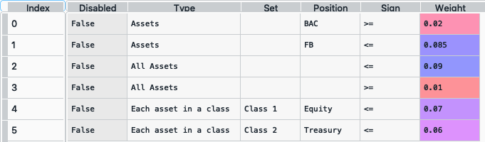
It is easier to construct the constraints in excel and then upload to a dataframe.

To create the pd.Series w_max and w_min we use the following command:

w_max, w_min = rp.hrp_constraints(constraints, asset_classes)

The pd.Series w_max and w_min looks like this (all constraints were merged to a single upper bound for each asset):

ConstraintsFunctions.risk_constraint(asset_classes, kind='vanilla', classes_col=None)[source]¶

Create the risk contribution constraint vector for the risk parity model.

Parameters:¶

asset_classes : DataFrame of shape (n_assets, n_cols)¶

Asset’s classes DataFrame, where n_assets is the number of assets and n_cols is the number of columns of the DataFrame where the first column is the asset list and the next columns are the different asset’s classes sets. It is only used when kind value is ‘classes’. The default value is None.

kind : str¶

Kind of risk contribution constraint vector. The default value is ‘vanilla’. Possible values are:

• ’vanilla’: vector of equal risk contribution per asset.

• ’classes’: vector of equal risk contribution per class.

classes_col : str or int¶

If value is str, it is the column name of the set of classes from asset_classes dataframe. If value is int, it is the column number of the set of classes from asset_classes dataframe. The default value is None.

Returns:¶

rb – The risk contribution constraint vector.

Return type:¶

nd-array

Raises:¶

ValueError when the value cannot be calculated. –

Examples

asset_classes = {'Assets': ['META', 'GOOGL', 'NFLX', 'BAC', 'WFC', 'TLT', 'SHV'],
                 'Class 1': ['Equity', 'Equity', 'Equity', 'Equity', 'Equity',
                              'Fixed Income', 'Fixed Income'],
                 'Class 2': ['Technology', 'Technology', 'Technology',
                              'Financial', 'Financial', 'Treasury', 'Treasury'],}

asset_classes = pd.DataFrame(asset_classes)
asset_classes = asset_classes.sort_values(by=['Assets'])
asset_classes.reset_index(inplace=True, drop=True)

rb = rp.risk_constraint(asset_classes
                        kind='classes',
                        classes_col='Class 1')

ConstraintsFunctions.connection_matrix(returns, custom_cov=None, codependence='pearson', graph='MST', walk_size=1, bins_info='KN', alpha_tail=0.05, gs_threshold=0.5)[source]¶

Create a connection matrix of walks of a specific size based on [E5] formula.

Parameters:¶

returns : DataFrame of shape (n_samples, n_assets)¶

Assets returns DataFrame, where n_samples is the number of observations and n_assets is the number of assets.

custom_cov : DataFrame or None, optional¶

Custom covariance matrix, used when codependence parameter has value ‘custom_cov’. The default is None.

codependence : str, can be {'pearson', 'spearman', 'abs_pearson', 'abs_spearman', 'distance', 'mutual_info', 'tail' or 'custom_cov'}¶

The codependence or similarity matrix used to build the distance metric and clusters. The default is ‘pearson’. Possible values are:

• ’pearson’: pearson correlation matrix. Distance formula: \(D_{i,j} = \sqrt{0.5(1-\rho^{pearson}_{i,j})}\).

• ’spearman’: spearman correlation matrix. Distance formula: \(D_{i,j} = \sqrt{0.5(1-\rho^{spearman}_{i,j})}\).

• ’kendall’: kendall correlation matrix. Distance formula: \(D_{i,j} = \sqrt{0.5(1-\rho^{kendall}_{i,j})}\).

• ’gerber1’: Gerber statistic 1 correlation matrix. Distance formula: \(D_{i,j} = \sqrt{0.5(1-\rho^{gerber1}_{i,j})}\).

• ’gerber2’: Gerber statistic 2 correlation matrix. Distance formula: \(D_{i,j} = \sqrt{0.5(1-\rho^{gerber2}_{i,j})}\).

• ’abs_pearson’: absolute value pearson correlation matrix. Distance formula: \(D_{i,j} = \sqrt{(1-|\rho_{i,j}|)}\).

• ’abs_spearman’: absolute value spearman correlation matrix. Distance formula: \(D_{i,j} = \sqrt{(1-|\rho_{i,j}|)}\).

• ’abs_kendall’: absolute value kendall correlation matrix. Distance formula: \(D_{i,j} = \sqrt{(1-|\rho^{kendall}_{i,j}|)}\).

• ’distance’: distance correlation matrix. Distance formula \(D_{i,j} = \sqrt{(1-\rho^{distance}_{i,j})}\).

• ’mutual_info’: mutual information matrix. Distance used is variation information matrix.

• ’tail’: lower tail dependence index matrix. Dissimilarity formula \(D_{i,j} = -\log{\lambda_{i,j}}\).

• ’custom_cov’: use custom correlation matrix based on the custom_cov parameter. Distance formula: \(D_{i,j} = \sqrt{0.5(1-\rho^{pearson}_{i,j})}\).

graph : string, optional¶

Graph used to build the adjacency matrix. The default is ‘MST’. Possible values are:

• ’MST’: Minimum Spanning Tree.

• ’TMFG’: Plannar Maximally Filtered Graph.

walk_size : int, optional¶

Size of the walk represented by the adjacency matrix. The default is 1.

bins_info : int or str¶

Number of bins used to calculate variation of information. The default value is ‘KN’. Possible values are:

• ’KN’: Knuth’s choice method. See more in knuth_bin_width.

• ’FD’: Freedman–Diaconis’ choice method. See more in freedman_bin_width.

• ’SC’: Scotts’ choice method. See more in scott_bin_width.

• ’HGR’: Hacine-Gharbi and Ravier’ choice method.

• int: integer value choice by user.

alpha_tail : float, optional¶

Significance level for lower tail dependence index. The default is 0.05.

gs_threshold : float, optional¶

Gerber statistic threshold. The default is 0.5.

Returns:¶

A_p – Adjacency matrix of walks of size lower and equal than ‘walk_size’.

Return type:¶

DataFrame

Raises:¶

ValueError when the value cannot be calculated. –

Examples

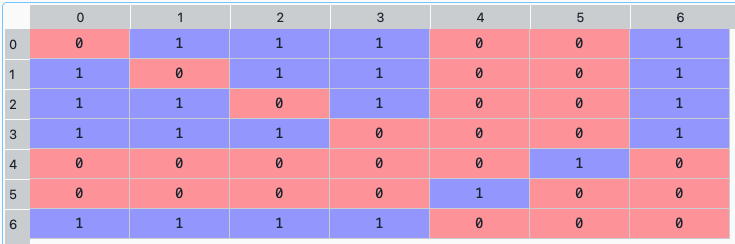
A_p = rp.connection_matrix(returns,
                           codependence="pearson",
                           graph="MST",
                           walk_size=1)

The connection matrix dataframe looks like the following image:

ConstraintsFunctions.centrality_vector(returns, measure='Degree', custom_cov=None, codependence='pearson', graph='MST', bins_info='KN', alpha_tail=0.05, gs_threshold=0.5)[source]¶

Create a centrality vector from the adjacency matrix of an asset network based on [E5] formula.

Parameters:¶

returns : DataFrame of shape (n_samples, n_assets)¶

Assets returns DataFrame, where n_samples is the number of observations and n_assets is the number of assets.

measure : str, optional¶

Centrality measure. The default is ‘Degree’. Possible values are:

• ’Degre’: Node’s degree centrality. Number of edges connected to a node.

• ’Eigenvector’: Eigenvector centrality. See more in eigenvector_centrality_numpy.

• ’Katz’: Katz centrality. See more in katz_centrality_numpy.

• ’Closeness’: Closeness centrality. See more in closeness_centrality.

• ’Betweeness’: Betweeness centrality. See more in betweenness_centrality.

• ’Communicability’: Communicability betweeness centrality. See more in communicability_betweenness_centrality.

• ’Subgraph’: Subgraph centrality. See more in subgraph_centrality.

• ’Laplacian’: Laplacian centrality. See more in laplacian_centrality.

custom_cov : DataFrame or None, optional¶

Custom covariance matrix, used when codependence parameter has value ‘custom_cov’. The default is None.

codependence : str, can be {'pearson', 'spearman', 'abs_pearson', 'abs_spearman', 'distance', 'mutual_info', 'tail' or 'custom_cov'}¶

The codependence or similarity matrix used to build the distance metric and clusters. The default is ‘pearson’. Possible values are:

• ’pearson’: pearson correlation matrix. Distance formula: \(D_{i,j} = \sqrt{0.5(1-\rho^{pearson}_{i,j})}\).

• ’spearman’: spearman correlation matrix. Distance formula: \(D_{i,j} = \sqrt{0.5(1-\rho^{spearman}_{i,j})}\).

• ’kendall’: kendall correlation matrix. Distance formula: \(D_{i,j} = \sqrt{0.5(1-\rho^{kendall}_{i,j})}\).

• ’gerber1’: Gerber statistic 1 correlation matrix. Distance formula: \(D_{i,j} = \sqrt{0.5(1-\rho^{gerber1}_{i,j})}\).

• ’gerber2’: Gerber statistic 2 correlation matrix. Distance formula: \(D_{i,j} = \sqrt{0.5(1-\rho^{gerber2}_{i,j})}\).

• ’abs_pearson’: absolute value pearson correlation matrix. Distance formula: \(D_{i,j} = \sqrt{(1-|\rho_{i,j}|)}\).

• ’abs_spearman’: absolute value spearman correlation matrix. Distance formula: \(D_{i,j} = \sqrt{(1-|\rho_{i,j}|)}\).

• ’abs_kendall’: absolute value kendall correlation matrix. Distance formula: \(D_{i,j} = \sqrt{(1-|\rho^{kendall}_{i,j}|)}\).

• ’distance’: distance correlation matrix. Distance formula \(D_{i,j} = \sqrt{(1-\rho^{distance}_{i,j})}\).

• ’mutual_info’: mutual information matrix. Distance used is variation information matrix.

• ’tail’: lower tail dependence index matrix. Dissimilarity formula \(D_{i,j} = -\log{\lambda_{i,j}}\).

• ’custom_cov’: use custom correlation matrix based on the custom_cov parameter. Distance formula: \(D_{i,j} = \sqrt{0.5(1-\rho^{pearson}_{i,j})}\).

graph : string, optional¶

Graph used to build the adjacency matrix. The default is ‘MST’. Possible values are:

• ’MST’: Minimum Spanning Tree.

• ’TMFG’: Plannar Maximally Filtered Graph.

bins_info : int or str¶

Number of bins used to calculate variation of information. The default value is ‘KN’. Possible values are:

• ’KN’: Knuth’s choice method. See more in knuth_bin_width.

• ’FD’: Freedman–Diaconis’ choice method. See more in freedman_bin_width.

• ’SC’: Scotts’ choice method. See more in scott_bin_width.

• ’HGR’: Hacine-Gharbi and Ravier’ choice method.

• int: integer value choice by user.

alpha_tail : float, optional¶

Significance level for lower tail dependence index. The default is 0.05.

gs_threshold : float, optional¶

Gerber statistic threshold. The default is 0.5.

Returns:¶

A_p – Adjacency matrix of walks of size ‘walk_size’.

Return type:¶

DataFrame

Raises:¶

ValueError when the value cannot be calculated. –

Examples

C_v = rp.centrality_vector(returns,
                           measure='Degree',
                           codependence="pearson",
                           graph="MST")

The neighborhood matrix looks like the following image:

ConstraintsFunctions.clusters_matrix(returns, custom_cov=None, codependence='pearson', linkage='ward', opt_k_method='twodiff', k=None, max_k=10, bins_info='KN', alpha_tail=0.05, gs_threshold=0.5, leaf_order=True)[source]¶

Creates an adjacency matrix that represents the clusters from the hierarchical clustering process based on [E6] formula.

Parameters:¶

returns : DataFrame of shape (n_samples, n_assets)¶

Assets returns DataFrame, where n_samples is the number of observations and n_assets is the number of assets.

custom_cov : DataFrame or None, optional¶

Custom covariance matrix, used when codependence parameter has value ‘custom_cov’. The default is None.

codependence : str, can be {'pearson', 'spearman', 'abs_pearson', 'abs_spearman', 'distance', 'mutual_info', 'tail' or 'custom_cov'}¶

The codependence or similarity matrix used to build the distance metric and clusters. The default is ‘pearson’. Possible values are:

• ’pearson’: pearson correlation matrix. Distance formula: \(D_{i,j} = \sqrt{0.5(1-\rho^{pearson}_{i,j})}\).

• ’spearman’: spearman correlation matrix. Distance formula: \(D_{i,j} = \sqrt{0.5(1-\rho^{spearman}_{i,j})}\).

• ’kendall’: kendall correlation matrix. Distance formula: \(D_{i,j} = \sqrt{0.5(1-\rho^{kendall}_{i,j})}\).

• ’gerber1’: Gerber statistic 1 correlation matrix. Distance formula: \(D_{i,j} = \sqrt{0.5(1-\rho^{gerber1}_{i,j})}\).

• ’gerber2’: Gerber statistic 2 correlation matrix. Distance formula: \(D_{i,j} = \sqrt{0.5(1-\rho^{gerber2}_{i,j})}\).

• ’abs_pearson’: absolute value pearson correlation matrix. Distance formula: \(D_{i,j} = \sqrt{(1-|\rho_{i,j}|)}\).

• ’abs_spearman’: absolute value spearman correlation matrix. Distance formula: \(D_{i,j} = \sqrt{(1-|\rho_{i,j}|)}\).

• ’abs_kendall’: absolute value kendall correlation matrix. Distance formula: \(D_{i,j} = \sqrt{(1-|\rho^{kendall}_{i,j}|)}\).

• ’distance’: distance correlation matrix. Distance formula \(D_{i,j} = \sqrt{(1-\rho^{distance}_{i,j})}\).

• ’mutual_info’: mutual information matrix. Distance used is variation information matrix.

• ’tail’: lower tail dependence index matrix. Dissimilarity formula \(D_{i,j} = -\log{\lambda_{i,j}}\).

• ’custom_cov’: use custom correlation matrix based on the custom_cov parameter. Distance formula: \(D_{i,j} = \sqrt{0.5(1-\rho^{pearson}_{i,j})}\).

linkage : string, optional¶

Linkage method of hierarchical clustering, see linkage for more details. The default is ‘ward’. Possible values are:

• ’single’.

• ’complete’.

• ’average’.

• ’weighted’.

• ’centroid’.

• ’median’.

• ’ward’.

• ’DBHT’. Direct Bubble Hierarchical Tree.

opt_k_method : str¶

Method used to calculate the optimum number of clusters. The default is ‘twodiff’. Possible values are:

• ’twodiff’: two difference gap statistic.

• ’stdsil’: standarized silhouette score.

k : int, optional¶

Number of clusters. This value is took instead of the optimal number of clusters calculated with the two difference gap statistic. The default is None.

max_k : int, optional¶

Max number of clusters used by the two difference gap statistic to find the optimal number of clusters. The default is 10.

bins_info : int or str¶

Number of bins used to calculate variation of information. The default value is ‘KN’. Possible values are:

• ’KN’: Knuth’s choice method. See more in knuth_bin_width.

• ’FD’: Freedman–Diaconis’ choice method. See more in freedman_bin_width.

• ’SC’: Scotts’ choice method. See more in scott_bin_width.

• ’HGR’: Hacine-Gharbi and Ravier’ choice method.

• int: integer value choice by user.

alpha_tail : float, optional¶

Significance level for lower tail dependence index. The default is 0.05.

gs_threshold : float, optional¶

Gerber statistic threshold. The default is 0.5.

leaf_order : bool, optional¶

Indicates if the cluster are ordered so that the distance between successive leaves is minimal. The default is True.

Returns:¶

A_c – Adjacency matrix of clusters.

Return type:¶

ndarray

Raises:¶

ValueError when the value cannot be calculated. –

Examples

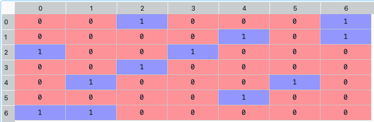
C_M = rp.clusters_matrix(returns,
                         codependence='pearson',
                         linkage='ward',
                         k=None,
                         max_k=10)

The clusters matrix looks like the following image:

ConstraintsFunctions.average_centrality(returns, w, measure='Degree', custom_cov=None, codependence='pearson', graph='MST', bins_info='KN', alpha_tail=0.05, gs_threshold=0.5)[source]¶

Calculates the average centrality of assets of the portfolio based on [E5] formula.

Parameters:¶

returns : DataFrame of shape (n_samples, n_assets)¶

Assets returns DataFrame, where n_samples is the number of observations and n_assets is the number of assets.

w : DataFrame or Series of shape (n_assets, 1)¶

Portfolio weights, where n_assets is the number of assets.

measure : str, optional¶

Centrality measure. The default is ‘Degree’. Possible values are:

• ’Degre’: Node’s degree centrality. Number of edges connected to a node.

• ’Eigenvector’: Eigenvector centrality. See more in eigenvector_centrality_numpy.

• ’Katz’: Katz centrality. See more in katz_centrality_numpy.

• ’Closeness’: Closeness centrality. See more in closeness_centrality.

• ’Betweeness’: Betweeness centrality. See more in betweenness_centrality.

• ’Communicability’: Communicability betweeness centrality. See more in communicability_betweenness_centrality.

• ’Subgraph’: Subgraph centrality. See more in subgraph_centrality.

• ’Laplacian’: Laplacian centrality. See more in laplacian_centrality.

custom_cov : DataFrame or None, optional¶

Custom covariance matrix, used when codependence parameter has value ‘custom_cov’. The default is None.

codependence : str, optional¶

The codependence or similarity matrix used to build the distance metric and clusters. The default is ‘pearson’. Possible values are:

• ’pearson’: pearson correlation matrix. Distance formula: \(D_{i,j} = \sqrt{0.5(1-\rho^{pearson}_{i,j})}\).

• ’spearman’: spearman correlation matrix. Distance formula: \(D_{i,j} = \sqrt{0.5(1-\rho^{spearman}_{i,j})}\).

• ’kendall’: kendall correlation matrix. Distance formula: \(D_{i,j} = \sqrt{0.5(1-\rho^{kendall}_{i,j})}\).

• ’gerber1’: Gerber statistic 1 correlation matrix. Distance formula: \(D_{i,j} = \sqrt{0.5(1-\rho^{gerber1}_{i,j})}\).

• ’gerber2’: Gerber statistic 2 correlation matrix. Distance formula: \(D_{i,j} = \sqrt{0.5(1-\rho^{gerber2}_{i,j})}\).

• ’abs_pearson’: absolute value pearson correlation matrix. Distance formula: \(D_{i,j} = \sqrt{(1-|\rho_{i,j}|)}\).

• ’abs_spearman’: absolute value spearman correlation matrix. Distance formula: \(D_{i,j} = \sqrt{(1-|\rho_{i,j}|)}\).

• ’abs_kendall’: absolute value kendall correlation matrix. Distance formula: \(D_{i,j} = \sqrt{(1-|\rho^{kendall}_{i,j}|)}\).

• ’distance’: distance correlation matrix. Distance formula \(D_{i,j} = \sqrt{(1-\rho^{distance}_{i,j})}\).

• ’mutual_info’: mutual information matrix. Distance used is variation information matrix.

• ’tail’: lower tail dependence index matrix. Dissimilarity formula \(D_{i,j} = -\log{\lambda_{i,j}}\).

• ’custom_cov’: use custom correlation matrix based on the custom_cov parameter. Distance formula: \(D_{i,j} = \sqrt{0.5(1-\rho^{pearson}_{i,j})}\).

graph : string, optional¶

Graph used to build the adjacency matrix. The default is ‘MST’. Possible values are:

• ’MST’: Minimum Spanning Tree.

• ’TMFG’: Plannar Maximally Filtered Graph.

bins_info : int or str¶

Number of bins used to calculate variation of information. The default value is ‘KN’. Possible values are:

• ’KN’: Knuth’s choice method. See more in knuth_bin_width.

• ’FD’: Freedman–Diaconis’ choice method. See more in freedman_bin_width.

• ’SC’: Scotts’ choice method. See more in scott_bin_width.

• ’HGR’: Hacine-Gharbi and Ravier’ choice method.

• int: integer value choice by user.

alpha_tail : float, optional¶

Significance level for lower tail dependence index. The default is 0.05.

gs_threshold : float, optional¶

Gerber statistic threshold. The default is 0.5.

Returns:¶

AC – Average centrality of assets.

Return type:¶

float

Raises:¶

ValueError when the value cannot be calculated. –

Examples

ac = rp.average_centrality(returns,
                           w,
                           measure="Degree"
                           codependence="pearson",
                           graph="MST")

ConstraintsFunctions.connected_assets(returns, w, custom_cov=None, codependence='pearson', graph='MST', walk_size=1, bins_info='KN', alpha_tail=0.05, gs_threshold=0.5)[source]¶

Calculates the percentage invested in connected assets of the portfolio based on [E5] formula.

Parameters:¶

returns : DataFrame of shape (n_samples, n_assets)¶

Assets returns DataFrame, where n_samples is the number of observations and n_assets is the number of assets.

w : DataFrame or Series of shape (n_assets, 1)¶

Portfolio weights, where n_assets is the number of assets.

custom_cov : DataFrame or None, optional¶

Custom covariance matrix, used when codependence parameter has value ‘custom_cov’. The default is None.

codependence : str, optional¶

The codependence or similarity matrix used to build the distance metric and clusters. The default is ‘pearson’. Possible values are:

• ’pearson’: pearson correlation matrix. Distance formula: \(D_{i,j} = \sqrt{0.5(1-\rho^{pearson}_{i,j})}\).

• ’spearman’: spearman correlation matrix. Distance formula: \(D_{i,j} = \sqrt{0.5(1-\rho^{spearman}_{i,j})}\).

• ’kendall’: kendall correlation matrix. Distance formula: \(D_{i,j} = \sqrt{0.5(1-\rho^{kendall}_{i,j})}\).

• ’gerber1’: Gerber statistic 1 correlation matrix. Distance formula: \(D_{i,j} = \sqrt{0.5(1-\rho^{gerber1}_{i,j})}\).

• ’gerber2’: Gerber statistic 2 correlation matrix. Distance formula: \(D_{i,j} = \sqrt{0.5(1-\rho^{gerber2}_{i,j})}\).

• ’abs_pearson’: absolute value pearson correlation matrix. Distance formula: \(D_{i,j} = \sqrt{(1-|\rho_{i,j}|)}\).

• ’abs_spearman’: absolute value spearman correlation matrix. Distance formula: \(D_{i,j} = \sqrt{(1-|\rho_{i,j}|)}\).

• ’abs_kendall’: absolute value kendall correlation matrix. Distance formula: \(D_{i,j} = \sqrt{(1-|\rho^{kendall}_{i,j}|)}\).

• ’distance’: distance correlation matrix. Distance formula \(D_{i,j} = \sqrt{(1-\rho^{distance}_{i,j})}\).

• ’mutual_info’: mutual information matrix. Distance used is variation information matrix.

• ’tail’: lower tail dependence index matrix. Dissimilarity formula \(D_{i,j} = -\log{\lambda_{i,j}}\).

• ’custom_cov’: use custom correlation matrix based on the custom_cov parameter. Distance formula: \(D_{i,j} = \sqrt{0.5(1-\rho^{pearson}_{i,j})}\).

graph : string, optional¶

Graph used to build the adjacency matrix. The default is ‘MST’. Possible values are:

• ’MST’: Minimum Spanning Tree.

• ’TMFG’: Plannar Maximally Filtered Graph.

walk_size : int, optional¶

Size of the walk represented by the adjacency matrix. The default is 1.

bins_info : int or str¶

Number of bins used to calculate variation of information. The default value is ‘KN’. Possible values are:

• ’KN’: Knuth’s choice method. See more in knuth_bin_width.

• ’FD’: Freedman–Diaconis’ choice method. See more in freedman_bin_width.

• ’SC’: Scotts’ choice method. See more in scott_bin_width.

• ’HGR’: Hacine-Gharbi and Ravier’ choice method.

• int: integer value choice by user.

alpha_tail : float, optional¶

Significance level for lower tail dependence index. The default is 0.05.

gs_threshold : float, optional¶

Gerber statistic threshold. The default is 0.5.

Returns:¶

CA – Percentage invested in connected assets.

Return type:¶

float

Raises:¶

ValueError when the value cannot be calculated. –

Examples

ca = rp.connected_assets(returns,
                         w,
                         codependence="pearson",
                         graph="MST",
                         walk_size=1)

ConstraintsFunctions.related_assets(returns, w, custom_cov=None, codependence='pearson', linkage='ward', opt_k_method='twodiff', k=None, max_k=10, bins_info='KN', alpha_tail=0.05, gs_threshold=0.5, leaf_order=True)[source]¶

Calculates the percentage invested in related assets based of the portfolio on [E6] formula.

Parameters:¶

returns : DataFrame of shape (n_samples, n_assets)¶

Assets returns DataFrame, where n_samples is the number of observations and n_assets is the number of assets.

w : DataFrame or Series of shape (n_assets, 1)¶

Portfolio weights, where n_assets is the number of assets.

custom_cov : DataFrame or None, optional¶

Custom covariance matrix, used when codependence parameter has value ‘custom_cov’. The default is None.

codependence : str, can be {'pearson', 'spearman', 'abs_pearson', 'abs_spearman', 'distance', 'mutual_info', 'tail' or 'custom_cov'}¶

The codependence or similarity matrix used to build the distance metric and clusters. The default is ‘pearson’. Possible values are:

• ’pearson’: pearson correlation matrix. Distance formula: \(D_{i,j} = \sqrt{0.5(1-\rho^{pearson}_{i,j})}\).

• ’spearman’: spearman correlation matrix. Distance formula: \(D_{i,j} = \sqrt{0.5(1-\rho^{spearman}_{i,j})}\).

• ’kendall’: kendall correlation matrix. Distance formula: \(D_{i,j} = \sqrt{0.5(1-\rho^{kendall}_{i,j})}\).

• ’gerber1’: Gerber statistic 1 correlation matrix. Distance formula: \(D_{i,j} = \sqrt{0.5(1-\rho^{gerber1}_{i,j})}\).

• ’gerber2’: Gerber statistic 2 correlation matrix. Distance formula: \(D_{i,j} = \sqrt{0.5(1-\rho^{gerber2}_{i,j})}\).

• ’abs_pearson’: absolute value pearson correlation matrix. Distance formula: \(D_{i,j} = \sqrt{(1-|\rho_{i,j}|)}\).

• ’abs_spearman’: absolute value spearman correlation matrix. Distance formula: \(D_{i,j} = \sqrt{(1-|\rho_{i,j}|)}\).

• ’abs_kendall’: absolute value kendall correlation matrix. Distance formula: \(D_{i,j} = \sqrt{(1-|\rho^{kendall}_{i,j}|)}\).

• ’distance’: distance correlation matrix. Distance formula \(D_{i,j} = \sqrt{(1-\rho^{distance}_{i,j})}\).

• ’mutual_info’: mutual information matrix. Distance used is variation information matrix.

• ’tail’: lower tail dependence index matrix. Dissimilarity formula \(D_{i,j} = -\log{\lambda_{i,j}}\).

• ’custom_cov’: use custom correlation matrix based on the custom_cov parameter. Distance formula: \(D_{i,j} = \sqrt{0.5(1-\rho^{pearson}_{i,j})}\).

linkage : string, optional¶

Linkage method of hierarchical clustering, see linkage for more details. The default is ‘ward’. Possible values are:

• ’single’.

• ’complete’.

• ’average’.

• ’weighted’.

• ’centroid’.

• ’median’.

• ’ward’.

• ’DBHT’. Direct Bubble Hierarchical Tree.

opt_k_method : str¶

Method used to calculate the optimum number of clusters. The default is ‘twodiff’. Possible values are:

• ’twodiff’: two difference gap statistic.

• ’stdsil’: standarized silhouette score.

k : int, optional¶

Number of clusters. This value is took instead of the optimal number of clusters calculated with the two difference gap statistic. The default is None.

max_k : int, optional¶

Max number of clusters used by the two difference gap statistic to find the optimal number of clusters. The default is 10.

bins_info : int or str¶

Number of bins used to calculate variation of information. The default value is ‘KN’. Possible values are:

• ’KN’: Knuth’s choice method. See more in knuth_bin_width.

• ’FD’: Freedman–Diaconis’ choice method. See more in freedman_bin_width.

• ’SC’: Scotts’ choice method. See more in scott_bin_width.

• ’HGR’: Hacine-Gharbi and Ravier’ choice method.

• int: integer value choice by user.

alpha_tail : float, optional¶

Significance level for lower tail dependence index. The default is 0.05.

gs_threshold : float, optional¶

Gerber statistic threshold. The default is 0.5.

leaf_order : bool, optional¶

Indicates if the cluster are ordered so that the distance between successive leaves is minimal. The default is True.

Returns:¶

RA – Percentage invested in related assets.

Return type:¶

float

Raises:¶

ValueError when the value cannot be calculated. –

Examples

ra = rp.related_assets(returns,
                       w,
                       codependence="pearson",
                       linkage="ward",
                       k=None,
                       max_k=10)

Bibliography

Fischer Black and Robert Litterman. Global portfolio optimization. Financial Analysts Journal, 48(5):28–43, 1992. URL: http://www.jstor.org/stable/4479577.
Wing Cheung. The augmented black-litterman model: a ranking-free approach to factor-based portfolio construction and beyond. Quantitative Finance, 13:, 08 2007. doi:10.2139/ssrn.1347648.
Petter Kolm and Gordon Ritter. On the bayesian interpretation of black-litterman. European Journal of Operational Research, 258:, 10 2016. doi:10.1016/j.ejor.2016.10.027.
Attilio Meucci. Fully flexible views: theory and practice. SSRN Electronic Journal, 2010. URL: https://papers.ssrn.com/sol3/papers.cfm?abstract_id=1213325.
Dany Cajas. A graph theory approach to portfolio optimization. SSRN Electronic Journal, 10 2023. doi:10.2139/ssrn.4602019.
Dany Cajas. A graph theory approach to portfolio optimization part ii. SSRN Electronic Journal, 12 2023. doi:10.2139/ssrn.4540021.